Run simulations
SuperDetectorPy contains scripts for both running simulations and visualizing the results. In this guide we go through how to run a simple simulation.
Run a simulation
Make sure to have a compiled mesh for the geometry that you wish to simulate. If you do not have any meshes, then follow the steps in this guide here.
Open a terminal, make sure to activate the SuperDetectorPy Anaconda environment (or the virtualenv), and navigate to the root fo the SuperDetectorPy repository. Run the following command after replacing RELATIVE_PATH_TO_MESH_FILE with the path to the mesh file:
python simulate.py RELATIVE_PATH_TO_MESH_FILE data/test-output.h5 -s 1e5 -t 0.01 -j 0.3 -J 0.4
The following parameters are used:
data/test-output.h5specifies the output file.-s 1e5run the simulation for \(1 \times 10^5\) time steps.-t 0.01run the simulation with time step \(0.01 \tau\).-j 0.3 -J 0.4interpolate the current density from \(0.3 J_0\) at the start of the simulation to \(0.4 J_0\) at the end of the simulation.
For information on how \(\tau\) and \(J_0\) are defined, please refer to section 2.2.1 in Theory for superconducting few-photon detectors.
Visualize the result
To visualize the results of the simulation run
python visualize.py data/test-output.h5
A Matplotlib window with the simulation results is opened. The following keys may be used to switch what is displayed:
right arrowjump to the next saved time step.left arrowjump to previous saved time step.shift + right arrowjump forward 10 saved time steps.shift + left arrowjump backwards 10 saved time steps.up arrowjump forward 100 saved time steps.down arrowjump backwards 100 saved time steps.shift + up arrowjump forward 1000 saved time steps.shift + down arrowjump backwards 1000 saved time steps.1display the amplitude of superconducting order parameter.2display the phase of superconducting order parameter.3display supercurrent density.4display normal current density.5display electrical scalar potential.6display magnetic vector potential.7display Ginzburg-Landau alpha parameter.
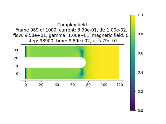
Fig. 2 A saved frame of the amplitude of the superconducting order parameter from the simulation above.
Fig. 2 depicts the amplitude of the superconducting order parameter when vortices enter the superconductor for the simulation ran in the previous section.
Warning
Quantities defined on the links between Voronoi sites (e.g. supercurrent and normal current) are not displayed correctly. The quantities vary slightly depending on the size and number of neighbours for each Voronoi site. This is not due to issues with the simulations, but rather due to difficulty to plot quantities defined on the dual mesh.